Developer Guide

This page provides a tutorial in the basics of using OP-PIC for unstructured-mesh PIC application development.

Example Application

The tutorial will use the FemPIC application, an electrostatic 3D unstructured mesh finite element PIC code (https://github.com/ExCALIBUR-NEPTUNE/Documents/blob/main/reports/2057699/TN-03-3.pdf).

It is based on tetrahedral mesh cells, nodes and faces forming a duct. Faces on one end of the duct are designated as inlet faces and the outer wall is fixed at a higher potential to retain the ions within the duct. Charged particles are injected at a constant rate from the inlet faces of the duct (one-stream) at a fixed velocity, and the particles move through the duct under the influence of the electric field. The particles are removed when they leave the boundary face. Overall Mini-FEM-PIC has 1 degree of freedom (DOF) per cell, 2 DOFs per node and 7 DOFs per particle.

FemPIC consists of six main loops, inject_ions , calculate_new_pos_vel , move , deposit_charge_on_nodes, compute_node_charge_density and compute_electric_field, within a time-marching iterative loop. Additionally, it contains a init_boundary_pot loop and a get_final_max_values loop used during initialzing and finalizing stages. In addition to the above loops, FemPIC consists of a linear sparse matrix field solver, which is implemented using PETSc library.

Out of these, compute_node_charge_density, init_boundary_pot and get_final_max_values are what we classify as direct loops where all the data accessed in the loop is defined on the mesh element over which the loop iterates over. Thus, for example in a direct loop, a loop over nodes will only access data defined on nodes.

All the other loops are indirect loops. In this case when looping over a given type of elements, data on other types of elements will be accessed indirectly, using mapping tables. There are two types of indirect loops. The compute_electric_field loop iterates over cells and read data on nodes, accessing them indirectly via a mapping table that gives the explicit connectivity information between cells and nodes. Similarly, calculate_new_pos_vel loop iterates over particles and read data on cells, accessing them indirectly via a mapping between particles and cells. The other kind of indirect loop is double-indirect. For example, deposit_charge_on_nodes loop iterates over particles and increments data on nodes. But these nodes are not directly related to particles though one mapping. Thus, we may need to use two mappings, the first from particles to cells (p2c_map) and the second from cells to nodes (c2n_map).

Within these above mentioned loop, there is a special loop which will move particles to cells according to the particle position, and the further details will be discussed in a later section.

• Go to the OP-PIC/app_fempic directory and open the fempic.cpp file to view the original application.

• Use the information in the readme file of that directory to code-generate and run the application.

Original - Load mesh and initialization

The original code begins with allocating memory to hold the mesh data and then initializing them by reading in the mesh data, form the text file.

In this tutorial, the main focus is to show how the OP-PIC API is used, hence the user may implement their own code for mesh loading.

Go to the OP-PIC/app_fempic/fempic_misc_mesh_loader.h to see the complete mesh loader, where we use the original Mini-FEM-PIC code to read from file and store in the data storage class DataPointers.

std::shared_ptr<DataPointers> m = load_mesh();

Step 1 - Preparing to use OP-PIC

First, include the following header files, then initialize OP-PIC and finalize it as follows:

#include "opp_templates.h"
...
...
int main(int argc, char **argv) {
    opp_init(argc, argv); //Initialise the OP-PIC library, passing runtime args
    {
        ...
        ...
        ...
    }
    opp_exit(); //Finalising the OP-PIC library
}

Step 2 - OP-PIC Declaration

(a) Declare sets

The FemPIC application consists of three mesh element types (which we call sets): cells, nodes, and inlet-faces. These needs to be declared using the opp_decl_set API call together with the number of elements for each of these sets.

In addition, FemPIC contains a particle set, that is defined using opp_decl_particle_set API call together with the number of particles and a mesh cell set.

The speciality of a particle set is that they can be resized (the set size can be increased or reduced during the simulation). Other than the main particle set, we have used a temporary dummy particle set to hold some random data for particle injection initialization.

// declare sets
opp_set node_set       = opp_decl_set(m->n_nodes, "mesh_nodes");
opp_set cell_set       = opp_decl_set(m->n_cells, "mesh_cells");
opp_set iface_set      = opp_decl_set(m->n_ifaces, "inlet_faces_cells");
opp_set particle_set   = opp_decl_particle_set("particles", cell_set);
opp_set dummy_part_set = opp_decl_particle_set("dummy particles", cell_set);

Later, we will see how the number of mesh elements can be read in directly from an hdf5 file using the opp_decl_set_hdf5 and opp_decl_particle_set_hdf5 call.

When developing your own application with OP-PIC, or indeed converting an application to use OP-PIC, you will need to decide on what mesh element types, i.e. sets will need to be declared to define the full mesh. A good starting point for this design is to see what mesh elements are used the loops over the mesh.

(b) Declare maps

Looking at the original Mini-FEM-PIC application’s loops we see that mappings between cells and nodes, cells and cells, inlet-faces and nodes, inlet-faces and cells, and cells and nodes are required. In addition, a particles to cells mapping is required.

This can be observed by the indirect access to data in each of the loops in the main iteration loops. These connectivity information needs to be declared via the opp_decl_map API call:

//declare maps
opp_map c2n_map  = opp_decl_map(cell_set,  node_set, 4, m->c_to_n, "c_v_n_map");
opp_map c2c_map  = opp_decl_map(cell_set,  cell_set, 4, m->c_to_c,  "c_v_c_map");
opp_map if2c_map = opp_decl_map(iface_set, cell_set, 1, m->if_to_c, "if_v_c_map");
opp_map if2n_map = opp_decl_map(iface_set, node_set, 4, m->if_to_n, "if_v_n_map");

opp_map p2c_map  = opp_decl_map(particle_set, cell_set, 1, nullptr, "p2c_map");

The opp_decl_map requires the names of the two sets for which the mapping is declared, its arity, mapping data (as in this case allocated in integer blocks of memory) and a string name. A map created with a particle set is capable of changing its length during the simulation and other maps are static.

Note that we have declared p2c_map with a nullptr since particle_set is defined without a particle count (i.e. zero), since we anticipate injecting particles during the simulation.

(c) Declare data

All data declared on sets should be declared using the opp_decl_dat API call. For FemPIC this consists of seven cell dats, six node dats, six inlet-face dats and three particle dats (+1 dummy particle dat).

//declare data on sets
  opp_dat c_det       = opp_decl_dat(cell_set, 16, DT_REAL, m->c_det,      "c_det");
  opp_dat c_volume    = opp_decl_dat(cell_set, 1,  DT_REAL, m->c_vol,      "c_volume");
  opp_dat c_ef        = opp_decl_dat(cell_set, 3,  DT_REAL, m->c_ef,       "c_ef");
  opp_dat c_sd        = opp_decl_dat(cell_set, 12, DT_REAL, m->c_sd,       "c_shape_deri");
  opp_dat c_gbl_id    = opp_decl_dat(cell_set, 1,  DT_INT,  m->c_id,       "c_gbl_id");
  opp_dat c_colors    = opp_decl_dat(cell_set, 1,  DT_INT,  m->c_col,      "c_colors");
  opp_dat c_centroids = opp_decl_dat(cell_set, 3,  DT_REAL, m->c_centroid, "c_centroids");

  opp_dat n_volume     = opp_decl_dat(node_set, 1, DT_REAL, m->n_vol,     "n_vol");
  opp_dat n_potential  = opp_decl_dat(node_set, 1, DT_REAL, m->n_pot,     "n_potential");
  opp_dat n_charge_den = opp_decl_dat(node_set, 1, DT_REAL, m->n_ion_den, "n_charge_den");
  opp_dat n_pos        = opp_decl_dat(node_set, 3, DT_REAL, m->n_pos,     "n_pos");
  opp_dat n_type       = opp_decl_dat(node_set, 1, DT_INT,  m->n_type,    "n_type");
  opp_dat n_bnd_pot    = opp_decl_dat(node_set, 1, DT_REAL, m->n_bnd_pot, "n_bnd_pot");

  opp_dat if_v_norm  = opp_decl_dat(iface_set, 3,  DT_REAL, m->if_v_norm, "iface_v_norm");
  opp_dat if_u_norm  = opp_decl_dat(iface_set, 3,  DT_REAL, m->if_u_norm, "iface_u_norm");
  opp_dat if_norm    = opp_decl_dat(iface_set, 3,  DT_REAL, m->if_norm,   "iface_norm");
  opp_dat if_area    = opp_decl_dat(iface_set, 1,  DT_REAL, m->if_area,   "iface_area");
  opp_dat if_distrib = opp_decl_dat(iface_set, 1,  DT_INT,  m->if_dist,   "iface_dist");
  opp_dat if_n_pos   = opp_decl_dat(iface_set, 12, DT_REAL, m->if_n_pos,  "iface_n_pos");

  opp_dat p_pos   = opp_decl_dat(particle_set, 3, DT_REAL, nullptr, "p_position");
  opp_dat p_vel   = opp_decl_dat(particle_set, 3, DT_REAL, nullptr, "p_velocity");
  opp_dat p_lc    = opp_decl_dat(particle_set, 4, DT_REAL, nullptr, "p_lc");

  opp_dat dp_rand = opp_decl_dat(dummy_part_set, 2, DT_REAL, nullptr, "dummy_part_rand");

Note that we have declared particle dats with a nullptr since particle_set is defined without a particle count (i.e. zero), since we anticipate injecting particles during the simulation.

(d) Declare constants

Finally global constants that are used in any of the computations in the loops needs to be declared. This is required due to the fact that when using code-generation later for parallelizations such as on GPUs (e.g. using CUDA or HIP), global constants need to be copied over to the GPUs before they can be used in a GPU kernel.

Declaring them using the opp_decl_const<type> API call will indicate to the OP-PIC code-generator that these constants need to be handled in a special way, generating code for copying them to the GPU for the relevant back-ends. The template types could be OPP_REAL, OPP_INT, OPP_BOOL.

//declare global constants
opp_decl_const<OPP_REAL>(1, &spwt,           "CONST_spwt");
opp_decl_const<OPP_REAL>(1, &ion_velocity,   "CONST_ion_velocity");
opp_decl_const<OPP_REAL>(1, &dt,             "CONST_dt");
opp_decl_const<OPP_REAL>(1, &plasma_den,     "CONST_plasma_den");
opp_decl_const<OPP_REAL>(1, &mass,           "CONST_mass");
opp_decl_const<OPP_REAL>(1, &charge,         "CONST_charge");
opp_decl_const<OPP_REAL>(1, &wall_potential, "CONST_wall_potential");

The constants can be accessed in the kernels with the same literals used in the string name. An example can be seen in the next section (Step 3).

Step 3 - Parallel loop : opp_par_loop

(a) Direct loop

We can now convert a direct loop to use the OP-PIC API.

We have chosen compute_node_charge_density to demostrate a direct loop. It iterates over nodes, multiply node_charge_den with (CONST_spwt / node_volume) and saves to multiply node_charge_den.

//compute_node_charge_density : iterates over nodes
for (int iteration = 0; iteration < (nnodes * 1); ++iteration) {
    node_charge_den[iteration] *= (CONST_spwt[0] / node_volume[iteration]);
}

This is a direct loop due to the fact that all data accessed in the computation are defined on the set that the loop iterates over. In this case the iteration set is nodes.

To convert to the OP-PIC API we first outline the loop body (elemental kernel) to a subroutine:

//outlined elemental kernel
inline void compute_ncd_kernel(double *ncd, const double *nv) {
    ncd[0] *= (CONST_spwt[0] / nv[0]);
}
//compute_node_charge_density : iterates over nodes
for (int iteration = 0; iteration < (nnodes * 1); ++iteration) {
    compute_ncd_kernel(&node_charge_den[iteration], &node_volume[iteration]);
}

Now we can directly declare the loop with the opp_par_loop API call:

//outlined elemental kernel
inline void compute_ncd_kernel(double *ncd, const double *nv) {
    ncd[0] *= (CONST_spwt[0] / nv[0]);
}

opp_par_loop(compute_ncd_kernel, "compute_node_charge_density", node_set, OPP_ITERATE_ALL,
    opp_arg_dat(n_charge_den,  OPP_RW),
    opp_arg_dat(n_volume,      OPP_READ));

Note how we have:

• indicated the elemental kernel compute_ncd_kernel in the first argument to opp_par_loop.

• used the opp_dat``s names ``n_charge_den and n_volume in the API call.

• noted the iteration set node_set (3rd argument) and iteration type OPP_ITERATE_ALL (4th argument).

• indicated the direct access of n_charge_den and n_volume without any mappings provided to opp_arg_dat.

• indicated that n_volume is read only (OP_READ) and n_charge_den is read & write (OPP_RW), by looking through the elemental kernel and identifying how they are used/accessed in the kernel.

• given that n_volume is read only we also indicate this by the key word const for compute_ncd_kernel elemental kernel.

• note that we have accessed a const value CONST_spwt that we declared using opp_decl_const<OPP_REAL>() API call.

(b) Indirect loop (single indirection)

We have selected two loops in FemPIC to demonstrate single indirections.

First, we use compute_electric_field calculation to showcase the mesh set to mesh set mapping indirections. Here we iterate over cells set, access node potentials through indirect accesses using c2n_map. Note that one cell in FemPIC is linked with 4 surrounding nodes and n_potential has a dimension of one.

//compute_electric_field : iterates over cells
for (int iter = 0; iter < ncell; ++iter) {
    const int map1idx = c2n_map[iter * 4 + 0];
    const int map2idx = c2n_map[iter * 4 + 1];
    const int map3idx = c2n_map[iter * 4 + 2];
    const int map4idx = c2n_map[iter * 4 + 3];

    for (int dim = 0; dim < 3; dim++) {
        c_ef[3 * iter + dim] = c_ef[12 * iter + dim] -
            ((c_sd[12 * iter + (0 + dim)] * n_potential[map1idx * 1 + 0])) +
            (c_sd[12 * iter + (3 + dim)] * n_potential[map2idx * 1 + 0])) +
            (c_sd[12 * iter + (6 + dim)] * n_potential[map3idx * 1 + 0])) +
            (c_sd[12 * iter + (9 + dim)] * n_potential[map4idx * 1 + 0])));
    }
}

Similar to the direct loop, we outline the loop body and call it within the loop as follows:

//outlined elemental kernel
inline void compute_ef_kernel(
    double *c_ef, const double *c_sd, const double *n_pot0,
    const double *n_pot1, const double *n_pot2, const double *n_pot3) {

    for (int dim = 0; dim < 3; dim++) {
        c_ef[dim] = c_ef[dim] -
            ((c_sd[0 + dim] * n_pot0[0])) + (c_sd[3 + dim] * n_pot1[0])) +
            (c_sd[6 + dim] * n_pot2[0])) + (c_sd[9 + dim] * n_pot3[0])));
    }
}
//compute_electric_field : iterates over cells
for (int iter = 0; iter < ncell; ++iter) {
    const int map1idx = c2n_map[iter * 4 + 0];
    const int map2idx = c2n_map[iter * 4 + 1];
    const int map3idx = c2n_map[iter * 4 + 2];
    const int map4idx = c2n_map[iter * 4 + 3];

    compute_ef_kernel(&c_ef[3 * iter], &c_sd[12 * iter], &n_potential[1 * map1idx],
        &n_potential[1 * map2idx], &n_potential[1 * map3idx], &n_potential[1 * map4idx]);
}

Now, convert the loop to use the opp_par_loop API:

//outlined elemental kernel
inline void compute_ef_kernel(
    double *c_ef, const double *c_sd, const double *n_pot0,
    const double *n_pot1, const double *n_pot2, const double *n_pot3) {

    for (int dim = 0; dim < 3; dim++) {
        c_ef[dim] = c_ef[dim] -
            ((c_sd[0 * 3 + dim] * n_pot0[0])) + (c_sd[1 * 3 + dim] * n_pot1[0])) +
            (c_sd[2 * 3 + dim] * n_pot2[0])) + (c_sd[3 * 3 + dim] * n_pot3[0])));
    }
}

opp_par_loop(compute_ef_kernel, "compute_electric_field", cell_set, OPP_ITERATE_ALL,
    opp_arg_dat(c_ef,                    OPP_RW),
    opp_arg_dat(c_sd,                    OPP_READ),
    opp_arg_dat(n_potential, 0, c2n_map, OPP_READ),
    opp_arg_dat(n_potential, 1, c2n_map, OPP_READ),
    opp_arg_dat(n_potential, 2, c2n_map, OPP_READ),
    opp_arg_dat(n_potential, 3, c2n_map, OPP_READ));

Note in this case how the indirections are specified using the mapping declared as opp_map c2n_map, indicating the to-set index (2nd argument), and access mode OPP_READ.

That is, the thrid argument of the opp_par_loop is a read-only argument mapped from cells to nodes using the mapping at the 0th index of c2n_map (i.e. 1st mapping out of 4 nodes attached). Likewise, the fourth argument of opp_par_loop is mapped from cells to nodes using the mapping at the 1st index of c2n_map (i.e. 2nd mapping out of 4 nodes attached) and so on.

Second, we use calculate_new_pos_vel calculation to showcase the particle set to mesh set mapping indirections. Here we iterate over particles set, access cell electric fields through indirect accesses using p2c_map. Note that one particle in FemPIC can be linked with only only one cell.

//calculate_new_pos_vel : iterates over cells
for (int iter = 0; iter < nparticles; ++iter) {
    const int p2c = p2c_map[iter];
    const double coef = CONST_charge[0] / CONST_mass[0] * CONST_dt[0];
    for (int dim = 0; dim < 3; dim++) {
        p_vel[3 * iter + dim] += (coef * c_ef[3 * p2c * dim]);
        p_pos[3 * iter + dim] += p_vel[3 * iter + dim] * CONST_dt[0];
    }
}

Then, we outline the loop body and call it within the loop as follows:

//outlined elemental kernel
inline void calc_pos_vel_kernel(
    const double *cell_ef, double *part_pos, double *part_vel) {

    const double coef = CONST_charge[0] / CONST_mass[0] * CONST_dt[0];
    for (int dim = 0; dim < 3; dim++) {
        part_vel[dim] += (coef * cell_ef[dim]);
        part_pos[dim] += part_vel[dim] * (CONST_dt[0]);
    }
}
//calculate_new_pos_vel : iterates over particles
for (int iter = 0; iter < nparticles; ++iter) {
    const int p2c = p2c_map[iter];
    calc_pos_vel_kernel(&c_ef[3 * p2c], &p_pos[3 * iter], &p_vel[3 * iter]);
}

Now, convert the loop to use the opp_par_loop API:

//outlined elemental kernel
inline void calc_pos_vel_kernel(
    const double *cell_ef, double *part_pos, double *part_vel) {

    const double coef = CONST_charge[0] / CONST_mass[0] * CONST_dt[0];
    for (int dim = 0; dim < 3; dim++) {
        part_vel[dim] += (coef * cell_ef[dim]);
        part_pos[dim] += part_vel[dim] * (CONST_dt[0]);
    }
}

opp_par_loop(calc_pos_vel_kernel, "calculate_new_pos_vel", particle_set, OPP_ITERATE_ALL,
    opp_arg_dat(c_ef, p2c_map, OPP_READ),
    opp_arg_dat(p_pos,         OPP_WRITE),
    opp_arg_dat(p_vel,         OPP_WRITE));

Note in this case how the indirections are specified using the mapping declared as opp_map p2c_map, and access mode OPP_READ.

That is, the first argument of the opp_par_loop is a read-only argument mapped from particles to cells, however a mapping index is not required since always particles to cells mapping has a dimension of one.

(c) Double Indirect loop

There could be instances where double indirection is required. For example in deposit_charge_on_nodes, we may need to deposit charge from particles to nodes, but from particles we have a single mapping towards the cells, with another mapping from cells to nodes.

Here we iterate over particles set, access node charge density through double-indirect accesses using p2c_map and c2n_map. Note that one cell in FemPIC is linked with 4 surrounding nodes and n_charge_den has a dimension of one.

//deposit_charge_on_nodes : iterates over cells
for (int iter = 0; iter < nparticles; ++iter) {
    const int p2c = p2c_map[iter];
    const int map1idx = c2n_map[p2c * 4 + 0];
    const int map2idx = c2n_map[p2c * 4 + 1];
    const int map3idx = c2n_map[p2c * 4 + 2];
    const int map4idx = c2n_map[p2c * 4 + 3];

    n_charge_den[1 * map1idx] += p_lc[4 * iter + 0];
    n_charge_den[1 * map2idx] += p_lc[4 * iter + 1];
    n_charge_den[1 * map3idx] += p_lc[4 * iter + 2];
    n_charge_den[1 * map4idx] += p_lc[4 * iter + 3];
}

Similarly, we outline the loop body and call it within the loop as follows:

//outlined elemental kernel
inline void dep_charge_kernel(const double *part_lc,
    double *node_charge_den0, double *node_charge_den1,
    double *node_charge_den2, double *node_charge_den3) {

    node_charge_den0[0] += part_lc[0];
    node_charge_den1[0] += part_lc[1];
    node_charge_den2[0] += part_lc[2];
    node_charge_den3[0] += part_lc[3];
}

//deposit_charge_on_nodes : iterates over cells
for (int iter = 0; iter < nparticles; ++iter) {
    const int p2c = p2c_map[iter];
    const int map1idx = c2n_map[p2c * 4 + 0];
    const int map2idx = c2n_map[p2c * 4 + 1];
    const int map3idx = c2n_map[p2c * 4 + 2];
    const int map4idx = c2n_map[p2c * 4 + 3];

    dep_charge_kernel(&p_lc[4 * iter],
        &n_charge_den[1 * map1idx], &n_charge_den[1 * map2idx],
        &n_charge_den[1 * map3idx], &n_charge_den[1 * map4idx]);
}

Now, convert the loop to use the opp_par_loop API:

//outlined elemental kernel
inline void dep_charge_kernel(const double *part_lc,
    double *node_charge_den0, double *node_charge_den1,
    double *node_charge_den2, double *node_charge_den3) {

    node_charge_den0[0] += part_lc[0];
    node_charge_den1[0] += part_lc[1];
    node_charge_den2[0] += part_lc[2];
    node_charge_den3[0] += part_lc[3];
}

opp_par_loop(dep_charge_kernel, "deposit_charge_on_nodes", particle_set, OPP_ITERATE_ALL,
    opp_arg_dat(p_lc,                              OPP_READ),
    opp_arg_dat(n_charge_den, 0, c2n_map, p2c_map, OPP_INC),
    opp_arg_dat(n_charge_den, 1, c2n_map, p2c_map, OPP_INC),
    opp_arg_dat(n_charge_den, 2, c2n_map, p2c_map, OPP_INC),
    opp_arg_dat(n_charge_den, 3, c2n_map, p2c_map, OPP_INC));

Note in this case how the indirections are specified using the mapping declared using two maps p2c_map and c2n_map, indicating the to-set index (2nd argument), and access mode OPP_INC.

That is, the second argument of the opp_par_loop is an increment argument mapped from particles to cells and cells to nodes using the mapping at the 0th index of c2n_map (i.e. 1st mapping out of 4 nodes attached). Likewise, the third argument of opp_par_loop is mapped from particles to cells and cells to nodes using the mapping at the 1st index of c2n_map (i.e. 2nd mapping out of 4 nodes attached) and so on.

Step 4 - Move loop : opp_particle_move

A key step in a PIC solver is the particle move. Here we will first illustrate how a particle mover operates in an unstructured mesh environment.

The main idea of a particle mover is to search and position particles once it is moved to a new position under the influence of electric and magnetic fields.

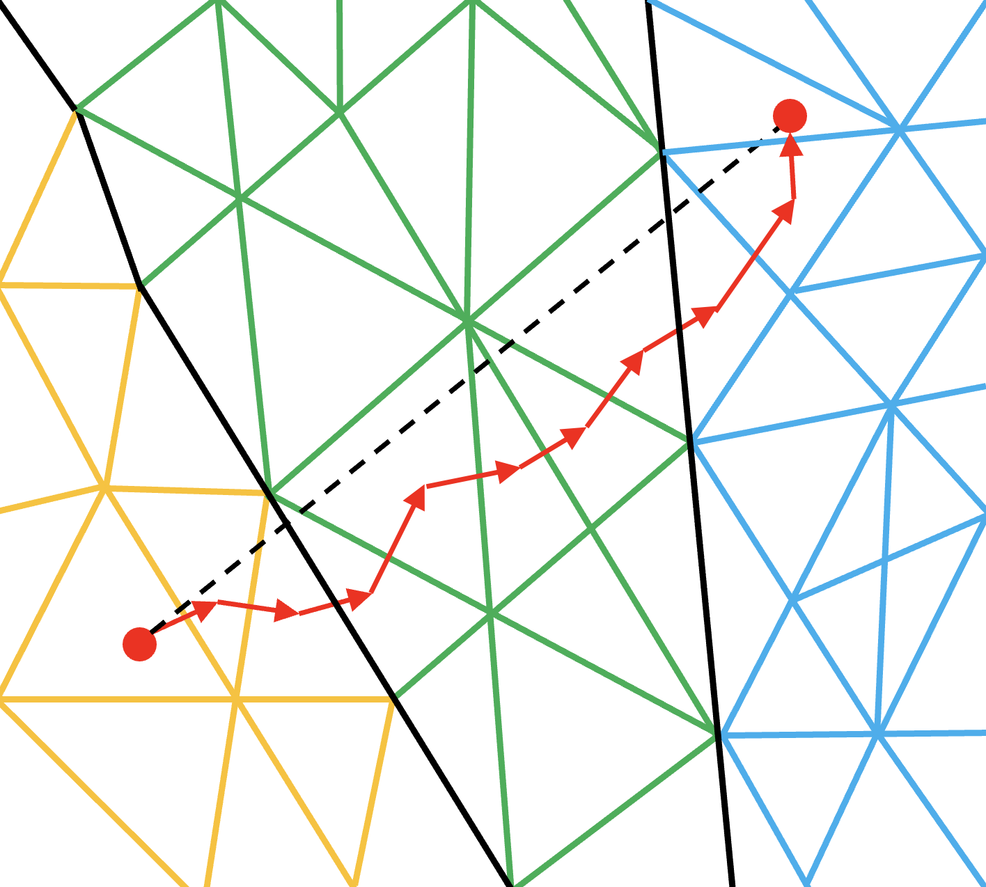
The first strategy that we discuss here is named as Multi-Hop (MH). It loop over each particle and “track” its movement from cell to cell by computing the next probable cell. This entails an inner loop per particle which will terminate when the final destination cell is reached.

To explain this, we use the FemPIC particle move routine.

//move_particles : iterates over cells
for (int iter = 0; iter < nparticles; ++iter) {

    bool search_next_cell = true;
    do {
        const int p2c = p2c_map[iter];
        const int c2c = c2c_map[4 * p2c];

        const double coeff = (1.0 / 6.0) / (c_volume[1 * p2c]);
        for (int i=0; i<4; i++) {
            p_lc[4 * iter + i] = coeff * (c_det[16 * p2c + i * 4 + 0] -
                c_det[16 * p2c + i * 4 + 1] * p_pos[3 * iter + 0] +
                c_det[16 * p2c + i * 4 + 2] * p_pos[3 * iter + 1] -
                c_det[16 * p2c + i * 4 + 3] * p_pos[3 * iter + 2]);
        }

        if (!(p_lc[4 * iter + 0] < 0.0 || p_lc[4 * iter + 0] > 1.0 ||
              p_lc[4 * iter + 1] < 0.0 || p_lc[4 * iter + 1] > 1.0 ||
              p_lc[4 * iter + 2] < 0.0 || p_lc[4 * iter + 2] > 1.0 ||
              p_lc[4 * iter + 3] < 0.0 || p_lc[4 * iter + 3] > 1.0)) { // within current cell
            search_next_cell = false;
        }
        else { // outside the last known cell
            int min_i = 0;
            double min_lc = p_lc[4 * iter + 0];

            for (int i=1; i < 4; i++) { // find most negative weight
                if (p_lc[4 * iter + i] < min_lc) {
                    min_lc = p_lc[4 * iter + i];
                    min_i = i;
                }
            }

            if (c2c_map[4 * p2c + min_i] >= 0) { // is there a neighbor in this direction?
                p2c_map[iter] = c2c_map[4 * p2c + min_i];
                search_next_cell = true;
            }
            else {
                // No neighbour cell to search next, particle out of domain,
                // Mark and remove from simulation!!!
                p2c_map[iter] = INT_MAX;
                search_next_cell = false;
            }
        }
    } while (search_next_cell)
}

Once this move routine is executed, there may be particles with INT_MAX p2c mapping, which means the data on all the particle dats related to that specific particle index are invalid.

One option is to fill these holes using valid particle data from the end of the array (we call it hole filling).

Another option is to sort all the particle arrays according to the p2c_map (desc), which will shift all particles with INT_MAX p2c mapping to shift to the end. This will have benefits of better cache usage, since all particles that maps to the same cell index will be close to each other, however, do note that sorting particle dats follow its own performance overhead!

One other option is to shuffle the particles, while shifting the particles with INT_MAX p2c mapping to the end of the data structure. The benefits of doing so in device implementations are elaborated in the Optimization section.

Similar to other parallel loops, we outline the loop body and call it within the loop as follows:

//outlined elemental kernel
inline void move_kernel(bool& search_next_cell, int* p2c, const int* c2c,
        const double *point_pos, double* point_lc,
        const double *cell_volume, const double *cell_det) {

    const double coeff = (1.0 / 6.0) / (cell_volume[0]);
    for (int i=0; i<4; i++) {
        point_lc[i] = coeff * (cell_det[i * 4 + 0] -
            cell_det[i * 4 + 1] * point_pos[0] +
            cell_det[i * 4 + 2] * point_pos[1] -
            cell_det[i * 4 + 3] * point_pos[2]);
    }

    if (!(point_lc[0] < 0.0 || point_lc[0] > 1.0 ||
          point_lc[1] < 0.0 || point_lc[1] > 1.0 ||
          point_lc[2] < 0.0 || point_lc[2] > 1.0 ||
          point_lc[3] < 0.0 || point_lc[3] > 1.0)) { // within the current cell
        search_next_cell = false;
        return;
    }

    // outside the last known cell
    int min_i = 0;
    double min_lc = point_lc[0];

    for (int i=1; i < 4; i++) { // find most negative weight
        if (point_lc[i] < min_lc) {
            min_lc = point_lc[i];
            min_i = i;
        }
    }

    if (c2c[min_i] >= 0) { // is there a neighbor in this direction?
        p2c[0] = c2c[min_i];
        search_next_cell = true;
    }
    else {
        // No neighbour cell to search next, particle out of domain,
        // Mark and remove from simulation!!!
        p2c[0] = INT_MAX;
        search_next_cell = false;
    }
}
//move_particles : iterates over cells
for (int iter = 0; iter < nparticles; ++iter) {

    bool search_next_cell = true;
    do {
        const int* p2c = &p2c_map[iter];
        const int* c2c = &c2c_map[4 * p2c[0]];

        move_kernel(search_next_cell, p2c, c2c,
            &p_pos[3 * iter], p_lc[16 * iter],
            &c_volume[1 * p2c[0]], &c_det[1 * p2c[0]]);

    } while (search_next_cell)
}

Now, convert the loop to use the opp_particle_move API.

//outlined elemental kernel
inline void move_kernel(const double *point_pos, double* point_lc,
        const double *cell_volume, const double *cell_det) {

    const double coeff = (1.0 / 6.0) / (cell_volume[0]);
    for (int i=0; i<4; i++) {                            // <- (1)
        point_lc[i] = coeff * (cell_det[i * 4 + 0] -
            cell_det[i * 4 + 1] * point_pos[0] +
            cell_det[i * 4 + 2] * point_pos[1] -
            cell_det[i * 4 + 3] * point_pos[2]);
    }

    if (!(point_lc[0] < 0.0 || point_lc[0] > 1.0 ||      // <- (2)
          point_lc[1] < 0.0 || point_lc[1] > 1.0 ||
          point_lc[2] < 0.0 || point_lc[2] > 1.0 ||
          point_lc[3] < 0.0 || point_lc[3] > 1.0)) { // within the current cell
        // no additional computations in FemPIC          // <- (3)
        OPP_PARTICLE_MOVE_DONE;
        return;
    }

    // outside the last known cell
    int min_i = 0;
    double min_lc = p_lc[0];

    for (int i=1; i < 4; i++) { // find most negative weight
        if (point_lc[i] < min_lc) {
            min_lc = point_lc[i];
            min_i = i;
        }
    }

    // is there a neighbor in this direction?
    if (opp_c2c[min_i] >= 0) {
        opp_p2c[0] = opp_c2c[min_i];                     // <- (5)
        OPP_PARTICLE_NEED_MOVE;
    }
    else {                                               // <- (4)
        // No neighbour cell to search next, particle out of domain,
        // Mark and remove from simulation!!!
        opp_p2c[0] = INT_MAX;
        OPP_PARTICLE_NEED_REMOVE;
    }
}

opp_particle_move(move_kernel, "move", particle_set, c2c_map, p2c_map,
    opp_arg_dat(p_pos,             OPP_READ),
    opp_arg_dat(p_lc,              OPP_WRITE),
    opp_arg_dat(c_volume, p2c_map, OPP_READ),
    opp_arg_dat(c_det,    p2c_map, OPP_READ));

Note how we have:

• indicated the elemental kernel move_kernel in the first argument to opp_particle_move loop.

• used particles_set as the iterating set and provided cell to cell mapping c2c_map and particle to cell mapping p2c_map as 4th and 5th arguments of the opp_particle_move API call.

• by providing c2c_map and p2c_map, they are accessed within the elemental kernel, using opp_c2c and opp_p2c pointers, without the need to explicitly pass as kernel arguments.

• direct, indirect, or double indirect mappings can be provided as opp_arg_dats similar to opp_par_loop (double indirection is not present in this example).

• OPP_PARTICLE_MOVE_DONE, OPP_PARTICLE_NEED_MOVE and OPP_PARTICLE_NEED_REMOVE pre-processor statements can be used to indicate the code-generator about the particle move status.

To summarize, the elemental kernel over all particles will require:

1. specifying computations to be carried out for each mesh element, e.g., cells, along the path of the particle, until its final destination cell.

2. a method to identify if the particle has reached its final mesh cell.

3. computations to be carried out at the final destination mesh cell.

4. actions to be carry out if the particle has moved out of the mesh domain.

5. calculate the next most probable cell index to search.

In additon to above, a user can provide a code-block to be executed only once per particle (during the first iteration of the do while loop) using the pre-processor directive OPP_DO_ONCE. This will be beneficial if the move kernel is required to include the code to calculate position and velocity (rather than a separate opp_par_loop like in FemPIC).

Additionally, if required deposit charge on nodes can be done at the place indicated by (3) in the elemental kernel.

inline void move_kernel(args ...) {
    if (OPP_DO_ONCE) {
        /* any computation that should get executed only once */
    }
    /* computation per mesh elment for particle */
    ...
    /* check condition for final destination */
    ...
    /* if final destination element - final computation*/
    OPP_PARTICLE_DONE_MOVE;
    ...
    /* else if out of domain*/
    OPP_PARTICLE_NEED_REMOVE;
    ...
    /* else - not final destination element - calculate next cell & move further*/
    OPP_PARTICLE_NEED_MOVE;
    ...
}

Once opp_particle_move is executed, all the particles that were marked as OPP_PARTICLE_NEED_REMOVE will get removed according to the routine requested by the user in the config file (hole-fill, sort, shuffle or a mix of these). More details on configs will be in a later section.

In addition, in an MPI and/or GPU target, all the communications and synchronizations will occur within opp_particle_move without any user intervention.

Eventhough, Multi-hop approach performs when particles move to closer cells, its performance is degraded when particles are moved to a faraway cell, making it to hop for long.

To address this issue of fast moving particles, OP-PIC incorporates a Direct-hop (DH) mechanism, where the particles are moved directly to a cell closer to the final destination, and then switches to multi-hop mode to move it to the correct final destination.

Note that, allthough, direct_hop reduces unnecessary computations and communications significantly, a higher memory footprint is required for bookkeeping.

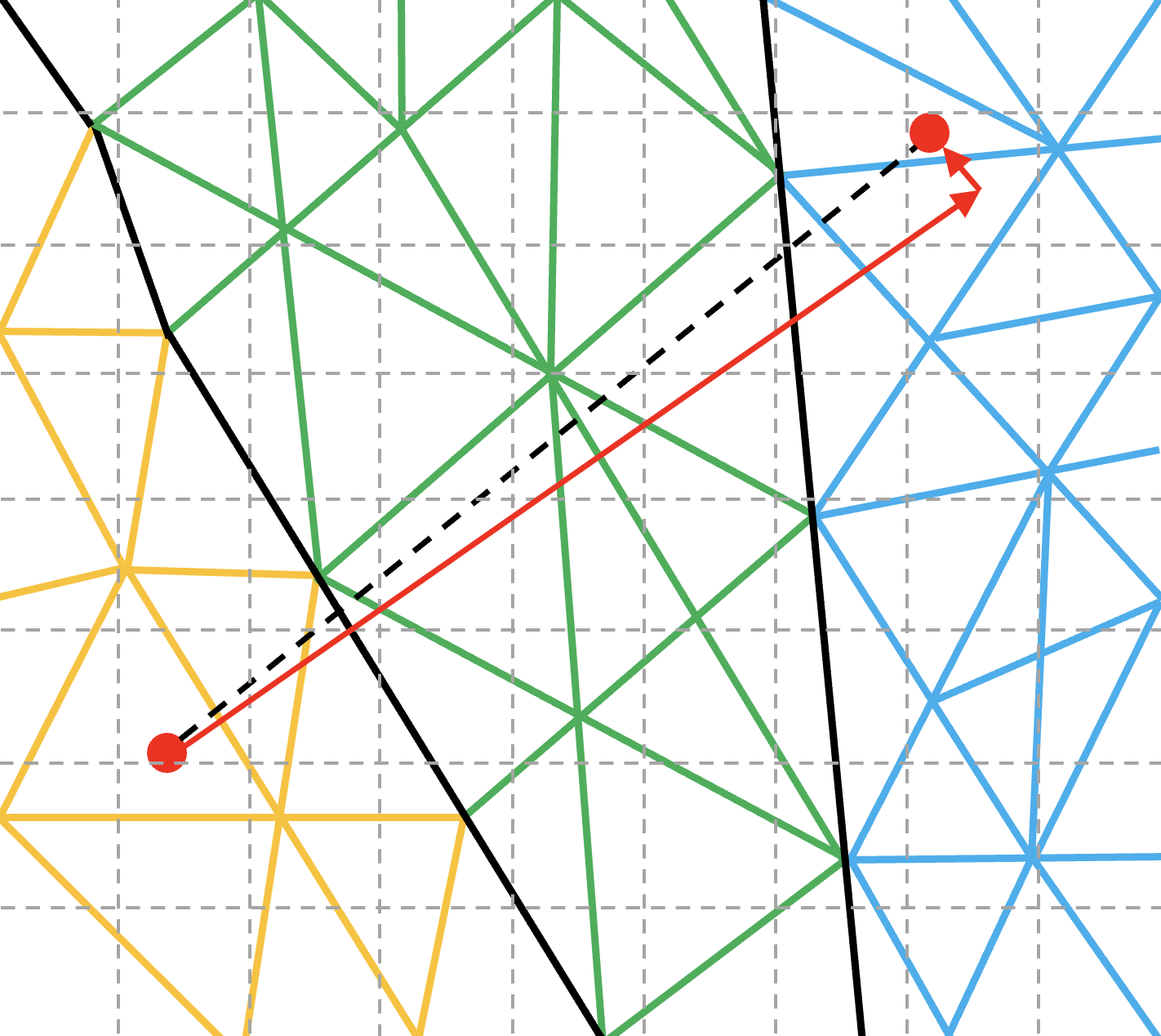
This mechanism can only be used in algorithms when it is not required to deposit contributions to all the passing cells during the particle movement. Hence, for the applications we tested, DH can be directly used for electro-static PIC codes, while electo-magnetic PIC codes require deposition of current to each passing cell.

To enable DH, the user should call the API opp_init_direct_hop, with the grid spacing (resolution) required in DH search scheme, dimension of the simulation (1D, 2D or 3D), a global cell index opp_dat (mainly required to translate cell indices in an MPI code simulation) and a opp::BoundingBox indicating the simulation boundaries.

opp_init_direct_hop(grid_spacing, DIM, c_gbl_id, bounding_box);

The bounding box can be created by providing a mesh dat that has its positions (like node positions) using:

opp::BoundingBox(const opp_dat pos_dat, int dim)

or simply by providing the calculated minimum and maximum domain coordinates using:

opp::BoundingBox(int dim, opp_point minCoordinate, opp_point maxCoordinate).

Once opp_init_direct_hop API is called, the code-generator will extract the required information from opp_particle_move API call, generate the initializing code for the additional data structures required for DH and change the internal do while loop to incorporate the additional DH algorithms.

However, even with an application having DH code generated and compiled, a user may wish to disable DH during runtime with no additional performance degradation to MH, using a config (discussed later).

Step 5 - Particle injections

In PIC simulations, particles can be initialized during setup stage, or can be injected during the simulation as an additional routine.

This particle injections imposes performance implications, since frequent reallocations takes time, especially in device code. To avoid this, OP-PIC introduces a new config opp_allocation_multiple (double) to pre-allocate the set with a multiple of its intended allocation size.

For example, if opp_allocation_multiple=10 and if the parts_to_insert=5,000, it will allocate space for 50,000 particles, making particle_set->set_capacity to 50,000 while maintaining particle_set->size at 5,000.

Hence during the injection of the second iteration of the main loop (assume parts_to_insert=5,000 again), it will simply make the particle_set->size to 10,000.

(a) Allocate space for particles

To allocate new particles, the API opp_increase_particle_count can be used. This will require the particle set to allocate and number of particles to insert.

void opp_increase_particle_count(opp_set p_set, int parts_to_insert)

Another API to inject particles is by, that requires particle distribution opp_dat. The part_dist dat should include the particle distribution per cell, and the p2c_map of the particle set will get enriched with the appropriate cell index.

void opp_inc_part_count_with_distribution(opp_set p_set, int parts_to_insert, opp_dat part_dist)

As an example, consider a mesh with 10 cells:

cell index	0	1	2	3	4	5	6	7	8	9
inject particles per cell	10	11	10	9	7	7	10	12	9	10
part_dist opp_dat	10	21	31	40	47	54	64	76	85	95

Since the mesh is unstructured mesh with different volumes, particles per cell can vary and part_dist opp_dat should have the particle counts as above (own particles + all particles prior to current cell index).

Providing this part_dist to opp_inc_part_count_with_distribution API call will enrich the p2c_map of first 10 particles with value 0, next 11 particles with value 1, following 10 particles wit value 2 and so on.

This will be beneficial in some cases where cell specific values need to be pre-known prior initializing particles (e.g. to get cell_ef to enrich p_vel).

(b) Initialize the injected particles

In order to initialize the injected particles, we can use opp_par_loop with iteration type of OPP_ITERATE_INJECTED. This will allow iterating only the particles that are newly injected.

However, once an opp_move_particle loop is executed, these particles will no longer be newly injected, hence a loop with OPP_ITERATE_INJECTED will not iterate any.

opp_par_loop(inject_ions_kernel, "inject_ions", particle_set, OPP_ITERATE_INJECTED,
    ... args ...
);

Step 6 - Global reductions

At this stage almost all the remaining loops can be converted to the OP-PIC API. Only the final loop get_final_max_values needs special handling due to its global reduction to get the max value of node charge density and node potential.

//get_final_max_values : iterates over nodes
double max_n_charge_den = 0.0, max_n_pot = 0.0;
for (int iter = 0; iter < nnodes; ++iter) {
    max_n_charge_den = MAX(abs(n_charge_den[1 * iter]), max_n_charge_den);
    max_n_pot = MAX(n_pot[1 * iter], max_n_pot);
}

Here, the global variable max_n_charge_den and max_n_pot are used as reduction variables. The kernel can be outlined as follows:

//outlined elemental kernel
inline void get_final_max_values_kernel(
    const OPP_REAL* n_charge_den, OPP_REAL* max_n_charge_den,
    const OPP_REAL* n_pot, OPP_REAL* max_n_pot) {
    max_n_charge_den = MAX(abs(n_charge_den[1 * iter]), max_n_charge_den);
    max_n_pot = MAX(n_pot[1 * iter], max_n_pot);
}
double max_n_charge_den = 0.0, max_n_pot = 0.0;
//get_final_max_values : iterates over nodes
for (int iter = 0; iter < nnodes; ++iter) {
    get_final_max_values_kernel(&n_charge_den[1 * iter], &max_n_charge_den,
                                &n_pot[1 * iter], &max_n_pot);
}

Now, convert the loop to use the opp_par_loop API:

//outlined elemental kernel
inline void get_final_max_values_kernel(
    const OPP_REAL* n_charge_den, OPP_REAL* max_n_charge_den,
    const OPP_REAL* n_pot, OPP_REAL* max_n_pot) {
    max_n_charge_den = MAX(abs(n_charge_den[1 * iter]), max_n_charge_den);
    max_n_pot = MAX(n_pot[1 * iter], max_n_pot);
}
double max_n_charge_den = 0.0, max_n_pot = 0.0;
opp_par_loop(get_final_max_values_kernel, "get_final_max_values", node_set, OPP_ITERATE_ALL,
    opp_arg_dat(n_charge_den,                   OPP_READ),
    opp_arg_gbl(&max_n_charge_den, 1, "double", OPP_MAX),
    opp_arg_dat(n_potential,                    OPP_READ),
    opp_arg_gbl(&max_n_pot,        1, "double", OPP_MAX));

This kind of global reductions can be done in both opp_par_loop and opp_particle_move loops.

At this point, all the loops have been converted to use opp_par_loop and opp_particle_move APIs. When developing applications for performance, you should consider freeing the initial memory allocated immediately after the relevant opp_decl_map and opp_decl_dat calls. In FemPIC, we are using m->DeleteValues() to free the initializing data structures.

In the next step we avoid freeing such “application developer allocated” memory by using HDF5 file I/O so that mesh data is directly read from file to OP-PIC allocated internal memory.

Step 7 - Handing it all to OP-PIC

Once the developer sequential version has been created and the numerical output validates the application can be prepared to obtain a developer distributed memory parallel version. This step can be completed to obtain a parallel executable that works with distributed memory MPI.

(a) Distributing data over MPI ranks

One way is to load the mesh into the OPP_ROOT (rank 0) and then distribute over MPI ranks. For an example, check distribute_data_over_ranks function in OP-PIC/app_fempic/fempic_misc_mesh_loader.h. This approach limits scaling when a large mesh is used (may take time to load data to one rank and distribute) and possibly run out of memory.

The other approach is to use HDF5 files to load data using HDF5 derivatives of the opp_decl_set, opp_decl_particle_set, opp_decl_map and opp_decl_dat API calls.

See OP-PIC/app_fempic/fempic_hdf5.cpp for a complete example.

opp_set node_set       = opp_decl_set_hdf5(file_name, "mesh_nodes");
opp_set cell_set       = opp_decl_set_hdf5(file_name, "mesh_cells");
opp_set iface_set      = opp_decl_set_hdf5(file_name, "inlet_faces_cells");
opp_set particle_set   = opp_decl_particle_set_hdf5(file_name, "particles", cell_set);
opp_set dummy_part_set = opp_decl_particle_set_hdf5(file_name, "dummy particles", cell_set);

opp_map c2n_map  = opp_decl_map_hdf5(cell_set,  node_set, 4, file_name, "c_v_n_map");
opp_map c2c_map  = opp_decl_map_hdf5(cell_set,  cell_set, 4, file_name, "c_v_c_map");
opp_map if2c_map = opp_decl_map_hdf5(iface_set, cell_set, 1, file_name, "if_v_c_map");
opp_map if2n_map = opp_decl_map_hdf5(iface_set, node_set, 4, file_name, "if_v_n_map");

opp_map p2c_map  = opp_decl_map(particle_set, cell_set, 1, nullptr, "part_mesh_rel");

opp_dat c_det       = opp_decl_dat_hdf5(cell_set, 16, DT_REAL, file_name, "c_det");
opp_dat c_volume    = opp_decl_dat_hdf5(cell_set, 1,  DT_REAL, file_name, "c_volume");
opp_dat c_ef        = opp_decl_dat_hdf5(cell_set, 3,  DT_REAL, file_name, "c_ef");
opp_dat c_sd        = opp_decl_dat_hdf5(cell_set, 12, DT_REAL, file_name, "c_shape_deri");
opp_dat c_gbl_id    = opp_decl_dat_hdf5(cell_set, 1,  DT_INT,  file_name, "c_gbl_id");
opp_dat c_colors    = opp_decl_dat_hdf5(cell_set, 1,  DT_INT,  file_name, "c_colors");
opp_dat c_centroids = opp_decl_dat_hdf5(cell_set, 3,  DT_REAL, file_name, "c_centroids");

opp_dat n_volume     = opp_decl_dat_hdf5(node_set, 1, DT_REAL, file_name, "n_vol");
opp_dat n_potential  = opp_decl_dat_hdf5(node_set, 1, DT_REAL, file_name, "n_potential");
opp_dat n_charge_den = opp_decl_dat_hdf5(node_set, 1, DT_REAL, file_name, "n_charge_den");
opp_dat n_pos        = opp_decl_dat_hdf5(node_set, 3, DT_REAL, file_name, "n_pos");
opp_dat n_type       = opp_decl_dat_hdf5(node_set, 1, DT_INT,  file_name, "n_type");
opp_dat n_bnd_pot    = opp_decl_dat_hdf5(node_set, 1, DT_REAL, file_name, "n_bnd_pot");

opp_dat if_v_norm  = opp_decl_dat_hdf5(iface_set, 3,  DT_REAL, file_name, "iface_v_norm");
opp_dat if_u_norm  = opp_decl_dat_hdf5(iface_set, 3,  DT_REAL, file_name, "iface_u_norm");
opp_dat if_norm    = opp_decl_dat_hdf5(iface_set, 3,  DT_REAL, file_name, "iface_norm");
opp_dat if_area    = opp_decl_dat_hdf5(iface_set, 1,  DT_REAL, file_name, "iface_area");
opp_dat if_distrib = opp_decl_dat_hdf5(iface_set, 1,  DT_INT,  file_name, "iface_dist");
opp_dat if_n_pos   = opp_decl_dat_hdf5(iface_set, 12, DT_REAL, file_name, "iface_n_pos");

opp_dat p_pos = opp_decl_dat_hdf5(particle_set, 3, DT_REAL, file_name, "part_position");
opp_dat p_vel = opp_decl_dat_hdf5(particle_set, 3, DT_REAL, file_name, "part_velocity");
opp_dat p_lc  = opp_decl_dat_hdf5(particle_set, 4, DT_REAL, file_name, "part_lc");

opp_dat dp_rand = opp_decl_dat_hdf5(dummy_part_set, 2, DT_REAL, file_name, "dummy_part_rand");

Note here that we assume that the mesh is already available as an HDF5 file and the name can be obtained as a config. (See the OP-PIC/app_handcoded/app_fempic_opphc/fempic_convert_hdf5.cpp utility application to understand how we can create an HDF5 file to be compatible with the OP-PIC API for FemPIC starting from mesh data defined in a text file.)

When the application has been switched to use the HDF5 API calls, manually allocated memory for the mesh elements can be removed. Additionally all printf statements should use opp_printf which will add details such as the MPI rank and main loop iteration count that this print statement is invoked. OPP_RUN_ON_ROOT() can be used to run only on root. We can also use timers, utilizing opp_profiler->start("name") and opp_profiler->end("name"), which will capture the time spent between these two calls and log it once the application calls opp_exit().

(b) Partitioning data over MPI ranks

Add the OP-PIC partitioner call opp_partition to the code in order to signal to the MPI back-end, the point in the program that all mesh data have been defined and mesh can be partitioned and MPI halos can be created. Even in the sequential execution this can be scoped between ifdef to avoid compilation issues.

...
...
opp_decl_const<OPP_REAL>(ONE, &wall_potential, "CONST_wall_potential");

#ifdef USE_MPI
    fempic_color_block(c_colors, c_centroids, if_n_pos, if2n_map);

    // opp_partition(std::string("PARMETIS_KWAY"), cell_set, c2n_map);
    // opp_partition(std::string("PARMETIS_GEOM"), iface_set, nullptr, if_n_pos);
    opp_partition(std::string("EXTERNAL"), cell_set, nullptr, c_colors);
#endif
...
...

See the API documentation for partitioner options.

In this case a special custom partitioning scheme is used to minimize particle communications. That is done by the enrichment of c_colors within a user written fempic_color_block function in OP-PIC/app_fempic/fempic_misc_mesh_colour.h.

Step 8 - Code generation

Now its time to generate the code for parallel versions. First we should move the elemental kernels to header files so that after the code generation the modified main application will not have the same elemental kernel definitions. This is only required since the code-generator removes the CONST_ global variables from the main c++ file (however, commenting a single line of code in code-generator will allow writing elemental kernels in the same c++ file).

Additionally, FemPIC requires a files solver that uses linear sparse matrix solving, hence we have implemented it as a separate PETSc based solver that can be found at:

OP-PIC/app_fempic/field_solver/

The complete regular and the HDF5 FemPIC applications can be found at OP-PIC/app_fempic/ which can be independently code generated using the below.

In general the below command can be used to code-generate.

python3 $OPP_TRANSLATOR -v -I$OPP_PATH/include/ --file_paths <application_cpp_file>

Specifically, for regular OP-PIC application without HDF5, use:

python3 $OPP_TRANSLATOR -v -I$OPP_PATH/include/ --file_paths fempic.cpp

If HDF5 is required, invoke the command:

python3 $OPP_TRANSLATOR -v -I$OPP_PATH/include/ --file_paths fempic_hdf5.cpp

Once the code-generator is invoked, a fempic_opp.cpp or fempic_hdf5_opp.cpp file and seq, omp, mpi, cuda and hip folders will be created, including a opp_kernels.<cpp|cu> file and a loop kernel header file per unique opp_par_loop or opp_particle_move loop per folder.